Using
Minimal Polynomial Bases for Model-Based Fault Diagnosis |
Vehicular Systems
group
Department of Electrical Engineering, Linkoping University
SE-581 83 Linkoping, Sweden
| To download the application in .pdf format (97 k), click here. |
| Introduction Theory Linear Residual Generation A Solution based on Minimal Polynomial Bases |
Finding the Minimal Polynomial Basis Design Example: Aircraft Dynamics References |
1 Introduction
A model based diagnosis
system commonly consists of a residual generator followed by thresholds and some
decision logic. The residual generator filters the known signals and generates a signal,
the residual, that should be small (ideally 0) in the fault-free case and large
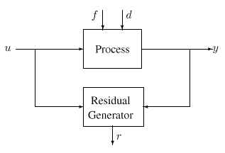
when a fault is acting on the system. In Figure 1, it is illustrated how the residual
generator is connected to the real system. The figure also shows that not only the control
signal u influences the system, but also disturbances d and the faults f that
we wish to detect. Both disturbances and faults are here modeled as input signals to
the system. In order not to make the residual sensitive to the disturbances d,
the disturbances must be decoupled. By using several residuals, or a vector-valued
residual, where not only disturbances but also different subset of faults are decoupled,
it is possible to achieve isolation. Isolation means distinguishing between different
faults and locate the fault component. This is the basic idea of a diagnosis system using
the principle of structured residuals (Gertler 1998) or the more general principle
of structured hypothesis tests (Nyberg 1999). The set of faults that, along with
the disturbances, are decoupled in a residual are called non-monitored faults.
Figure 1: A residual generator.
2 Theory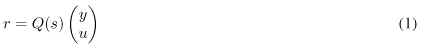
2.1 Linear Residual Generation
The systems studied in this work are assumed to be on the form
where y(t) is measurements, u(t) is known inputs to the system, d(t) is unknown disturbances including non-monitored faults, and f(t) is the monitored faults. The filter Q(s) in (1) is a residual generator if and only if the transfer function from u and d to r is zero, i.e. limt !1 r(t) = 0 for all d(t) and u(t) when f(t) = 0. To be able to detect faults, it is also required that r(t) <> 0 when f(t) <> 0.
Inserting (2) into (1) gives
![]()
To make r(t) = 0 when f(t) = 0, it is required that disturbances and the control signal are decoupled, i.e. for Q(s) to be a residual generator, it must hold that
![]()
Also, it is required that
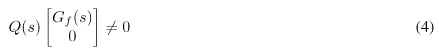
with suitable properties, e.g. adequate DC-gain from faults. Thus, the linear residual generation problem is to find a suitable Q(s) that fulfills (3) and (4).
2.2 A Solution based on Minimal
Polynomial Bases
This null-space is denoted NL(M(s)). The matrix Q(s) thus need to fulfill two requirements: belong to the left null-space of M(s) and give good fault sensitivity properties in the residual. If, in a first step of the design, all Q(s) that fulfills the first requirement is found, then a Q(s) with good fault sensitivity properties can be selected. Thus, in a first step of the design of the residual generator Q(s) we need not consider f or Gf (s). The problem is then to find all rational Q(s) that belong to NL(M(s)). Of special interest are the residual generators with least McMillan degree, i.e. the number of states in a minimal realization. Finding all Q(s) in NL(M(s)) can be done by finding a minimal basis for the rational vector-space NL(M(s)). A minimal basis for a rational vector-space is a polynomial basis (Forney 1975). For now, assume that such a basis can be found and let the base vectors be the rows of a matrix denoted NM(s). How to extract such a basis will be dealt with in Section 2.3. By inspection of (5), it can be realized that the dimension of NL(M(s)) (i.e. the number of rows of NM(s) is
where m is the number of outputs, i.e. the dimension of y(t), and kd is the number of disturbances, i.e. the dimension of d(t). The last equality holds only if rank Gd(s) = kd, but this should be the normal case. When a polynomial basis NM(s) has been obtained, the second and final step in the residual generator design is to shape fault-to-residual responses as described next. The minimal polynomial basis NM(s) is irreducible and because of this (Kailath 1980), all decoupling residual generators Q(s) can be parameterized as
where (s) is an arbitrary rational vector of
suitable dimensions. This parameterization vector
(s) can e.g. be used to shape the
fault-to-residual response or simply to select one row in . Since NM(s)
is a basis, the parameterization vector
(s) have minimal number of elements. The only
constraint on
![]() (s)
if the residual generator Q(s) is to be realizable, it must be chosen such
that (6) is proper. This means that the dynamics, i.e. poles, of the residual generator Q(s)
can be chosen freely. This also means that the minimal order of a realization of a
decoupling filter is determined by the row-degrees of the minimal polynomial basis NM(s).
(s)
if the residual generator Q(s) is to be realizable, it must be chosen such
that (6) is proper. This means that the dynamics, i.e. poles, of the residual generator Q(s)
can be chosen freely. This also means that the minimal order of a realization of a
decoupling filter is determined by the row-degrees of the minimal polynomial basis NM(s).
2.3 Finding the Minimal Polynomial Basis
The problem of finding a minimal polynomial basis to the left null-space of
the rational matrix M(s) can be solved by a transformation to a problem of
finding a minimal polynomial basis to the left null space of a polynomial matrix. This
transformation can be done in several different ways. In this section, two possibilities
are demonstrated, where one is used if the model is given on transfer function form and
the other if the model is given in state-space form. The motivation for this
transformation to a purely polynomial problem, is that there exists well established
theory (Kailath 1980) for polynomial matrices. In addition, the generally available
software, (The Polynomial Toolbox 2.0 for Matlab 5 1998), contains an extensive set
of tools for numerical handling of polynomial matrices.
State-Space Solution
Assume that the system is described in state-space form,
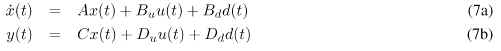
Then it is convienient to use the system matrix in state-space form (Rosenbrock 1970) to find the left null-space to M(s). Denote the system matrix Ms(s), describing the system with disturbances as inputs:
![]()
Also define the matrix P as
![]()
Then the following theorem gives a direct method on how to find a minimal polynomial basis to
NL(M(s)) via the system matrix.Theorem 1. Let V (s) be a minimal polynomial basis for
NL(M(s)) and let the pair { A, [Bu Bd] } be controllable. Then W(s) = V (s)P is a minimal polynomial basis for NL(M(s)).The proof of this theorem can be found in (Frisk & Nyberg 1999a). In conclusion, the problem of finding a minimal polynomial basis to a general rational matrix has been transformed into finding a minimal polynomial basis to a specific matrix pencil, in this case the system matrix Ms(s).
Frequency Domain Solution
If the model is given on transfer function form, one way of transforming the rational
problem to a polynomial problem is to perform a right MFD on M(s), i.e.
![]()
One simple example is
![]()
where d(s) is the least common multiple of all denominators. By finding a polynomial basis for the left null-space of the polynomial matrix M1(s), a basis is found also for the left null-space of M(s). No solutions are missed because D(s) (e.g. d(s)) is of full normal rank. Thus the problem of finding a minimal polynomial basis to
NL(M(s)) has been transformed into finding a minimal polynomial basis to3 Design Example: Aircraft Dynamics
This model, taken from (Maciejowski 1989), represents a linearized model of
vertical-plane dynamics of an aircraft. This section includes MATLAB code of central
operations. The inputs and outputs of the model are
The following Matlab-code defines model equations:
%% Define state-space matrices
>> A = [0, 0, 1.1320, 0,-1
0,-0.0538,-0.1712,
0,0.0705
0, 0, 0, 1,0
0, 0.0485,
0,-0.8556,-1.0130
0,-0.2909, 0,
1.0532,-0.6859];
>> B = [0,0,0
-0.1200,1,0
0,0,0
4.4190,0,-1.6650
1.5750,0,-0.0732];
>> C = [eye(3)
zeros(3,2)];
>> D = zeros(3,3);
Suppose the faults of interest are sensor-faults (denoted f1 , f2 , and f3 ), and actuator-faults (denoted f4 , f5 , and f6 ). Also, assume that the faults are modeled with additive fault models. The total model, including fault models then becomes:
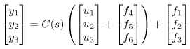
where
![]()
Thus, the transfer function from fault vector f to measurement vector y becomes, Gyf (s) = [I3 G(s)]. The design example is to design a residual generator Q(s) that decouples faults in the elevator angle actuator, i.e. f6 is considered a disturbance during the design. The matrix Gd(s) from Equation 2 corresponds to all signals that are to be decoupled, i.e. considered disturbances. In this case, Gd(s) becomes the column in Gyf (s) corresponding to f6 , i.e. the third column in G(s). Matrix Gf(s) corresponds to the monitored faults and therefore Gf(s) becomes the rest of the columns of Gyf (s). The following Matlab-code defines the transferfunctions from faults and disturbances.
>> Gd = Gu(:,3);
>> Gyf = [eye(3,3) Gu];
>> ndist = size(Gd,2);
>> nfault = size(Gyf,2);
The next step in the design is to find NM(s). Before using Theorem 1, the controllability requirement needs to be checked. Matlab gives
>> B_d = B(:,3);
>> D_d = D(:,3);
>> rank(ctrb(A,[B B_d]))
ans =
5
i.e. the controllability requirement is fulfilled. The Polynomial Toolbox macro null (computation of the right null-space of a polynomial matrix) can then be used to compute the required left null-basis with the help of the transpose operator
>> Ms = [C D_d;-(s*eye(n)-A) B_d)];
>> P = [eye(nmeas) -D;zeros(n,nmeas) -B];
The second method, the frequency domain approach can also be used. Direct calculations give
>> M = minreal([Gu
Gd;eye(nctrl) zeros(nctrl,ndist)]);
>> [N,D] = ss2rmf(M.a, M.b, M.c, M.d);
>> Nm2 = null(N.’).’
Nm2 =
0.071s 0.054 + s 0.091 0.12 -1 0
15s + 23sˆ2 -6.7 -17 - 0.94s + sˆ2 31 0 0
where ss2rmf is a macro of the Polynomial Toolbox that converts a state-space model to a right MFD. As can be seen, the bases are identical. A minimal polynomial basis is not unique, but the algorithm implemented in the toolbox null command is based on a canonical echelon form resulting in identical bases. The above basis has a natural interpretation. It means that the following equations hold in the fault-free case and also for all values of the actuator fault f6 = d.

The final step in the design is to choose the parametrization vector '(s). In a first design, utilize the first relation (9) and add low-pass dynamics by setting
![]()
Matlab-code to form the residual generator:
>> [Qa,Qb,Qc,Qd] =
lmf2ss([1,0]*Nm,s+1);
>> Q = ss(Qa,Qb,Qc,Qd);
![]()
It is clear that the decoupling has suceeded, down to machine precision, and that there is a nonzero gain from all faults besides f6 which was to be decoupled. Since the null-space had two basis vectors, we have some freedom in using both these relationships, i.e. (9) and (10), to form the residual generator. By letting
![]()
i.e. use a linear combination of the two basis vectors and add 2nd order low-pass dynamics to form the residual generator. Here, at least a 2nd order low-pass link was needed since the row-degree of the second basis vector was 2. The residual generator is also normed to have the same DC-gain as the first design to be able to do some comparison. Matlab-code to form the residualgenerator:
>> [Q2a,Q2b,Q2c,Q2d] =
lmf2ss([1,-1]*Nm,(s+1)ˆ2);
>> Q2 = ss(Q2a,Q2b,Q2c,Q2d);
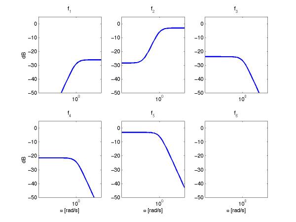
Evaluation of decoupling and fault sensitivity properties of this second design is shown in Figures 3 where fault sensitivity is shown. calculating
![]()
shows that the decoupling, also here has succeded down to machine precision. This second design shows how the design freedom available in '(s) can be used to shape important transfer functions and still keep the important decoupling property.
Figure 2: Transfer functions from the 6 faults to the residual. Note that fault 6 is decoupled, i.e. gain 0 from f6 to r.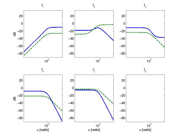
Forney, G. (1975). Minimal bases of rational vector spaces, with applications to multivariable linear systems, SIAM J. Control 13(3): 493–520.
Frisk, E. & Nyberg, M. (1999a). A description of the minimal polynomial basis approach to linear residual generation, Technical Report LiTH-R-2088, ISY, Linkoping, Sweden.
Frisk, E. &Nyberg, M. (1999b). Using minimal polynomial bases for fault diagnosis, European Control Conference, Karlsruhe, Germany.
Gertler, J. (1998). Fault Detection and Diagnosis in Engineering Systems, Marcel Dekker.
Kailath, T. (1980). Linear Systems, Prentice-Hall.
Maciejowski, J. (1989). Multivariable Feedback Design, Addison Wesley.
Nyberg, M. (1999). Framework and method for model based diagnosis with application to an automotive engine, European Control Conference.
Nyberg, M. & Frisk, E. (1999). A minimal polynomial basis solution to residual generation for fault diagnosis in linear systems, Vol. P, IFAC, Beijing, China, pp. 61–66.
Patton, R., Frank, P. & Clark, R. (eds) (1989). Fault diagnosis in Dynamic systems, Systems and Control Engineering, Prentice Hall.
Rosenbrock, H. (1970). State-Space and Multivariable Theory, Wiley, New York.
The Polynomial Toolbox 2.0 for Matlab 5 (1998). Polyx, Czech Republic. URL: http://www.polyx.com.